physical sun

Animated clouds with mental ray Physical Sky – Tutorial

In general the trick is to add the clouds (either an image or a node) to the physical sky “Haze” value as Master Zap indicated in his blog.

To achive that in Maya you will need the following.
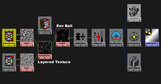
Maya nodes = noise, multiplyDivide and luminance.

Connect as follow
noise out color > multiplyDivide input
multiplyDivide output > luminance input
luminance out value > mia_physicalsky haze.

The noise node will serve as the clouds in the sky, which can be animated easily.

Once rendered you will hardly notice any clouds.

This where the multiply/divide nodes comes in.
Increase “Input 2″ to be 20, 0, 0
Now you will have more prominent clouds.

Since the haze parameter accept only ONE value.
The RGB > Luminance node can be useful in this connection, since it will convert the 3 out values of RGB to 1 value which is luminance.

In the Noise node, you can animate the time value to get the animated clouds in your render.

Note: The Noise node can be replaced with a texture file or any other Maya nodes.

To achieve more realistic result, add an envBall node to the shading network, this will give the sky roundness effect rather than just a flat image.

From here you can start building more complicated network to get more realistic look.

Note: to get rid of these artifacts that you see on the cone object, one needs to examine the network connection closely.
The clouds were connected to the “haze” parameter, however that “Sky haze” is already connected to the “Sun haze”

Once this connection is broken, the artifacts will disappear, however you will need test it since this test was made on a simple scene and it might have a side effect in an actual production file.

The following image reminds me with Alias Power Animator Sky system.
If you know what I’m talking about , then you are old.

Note:

Another photoreal tutorial

Making of Male Green Frog

Author: Massimo Righi

Software: Autodesk Maya

Author Website: http://www.massimorighi.com/

Hi, my name is Massimo Righi and I am a freelance CG artist from Italy.

What I'm going to do is try and show you the main steps of how I made my "Male Green Frog" image. I used Maya 8 for modelling, MentalRay for rendering and Photoshop for the textures.

The goal for me was to not only create a photo-realistic render, but also a 3d model for animation purposes, without the use of ZBrush (or similar software) and without adding any kind of post-work to the final render.

The first thing was to do some research to find some good references, having in mind the final result I wanted to achieve. I wasn't able to find all the views of the same frog that I wanted, so I mixed a lot of different frogs in order to model the main shape.

I started building the low-poly frog using a simple polygon plane and extruded the edges following the reference pics. I then modelled the main body leaving holes where the legs were to be connected.

After that, I created the legs and then joined them to the body.

As you can see from the WIP pic below, I've built only half of the frog so that I had only half of the UV map to deal with.

For the main (half) body and the leg, I made 2 cylindrical maps and for the feet I used 2 planar maps: 1 from the top view and one from bottom view. I used a simple checker applied to a lambert shader for checking the overall process while tweaking the UVs.

After that, I duplicated the half and combined everything together, ending up with 1.960 polygons, which is quite good for the low poly model (this then can be used as a cage for the rigging/animation process).

I than duplicated the frog keeping the low model in another layer, and then made the higher poly version (about 30.000 poly) doing a polysmooth. Finally, I added some details using the Maya sculpting tools, trying always to follow the main reference.

Using photos and freehand (I used a Wacom tablet), I made the textures in Photoshop each 2048x2048. Then I applied the texture to the frog, but I did notice (I was expecting that ) that some of the texture seams needed to be adjusted. So I used the built-in Maya 3d paint for that, using the clone tool.

When the color texture was made, I created the specular, bump and diffuse maps from it.

Now was the time for setting up the scene. I created a simple plane where I placed the frog and rotated it about 17° (I've done the same for the frog too). For the plane texture, I used a photo made by me and cropped it to about 1300x900... then I made the bump.

I created a camera and enabled the depth of field on it. As you can see from the grab, I made a distance tool placing one locator in the point of focus on the model and the other locator in the camera lens. I than parented that locator to the camera so that when I was moving the camera, the dimension value was also changing.

Before working on lighting, I made the shader networks; one for the main frog and one for the eyeballs. After some render tests, I decided to use a blinn shader with a Translucence value=1 for both.

For the lighting setup, I used an HDRI probe and 3 lights: 1 point-light (raytrace shadow) and 2 spotlights.

For the MentalRay render settings, I used a mitchell filter with a sample level min=1 max=3, Ray tracing and Final-Gather.

Here is the final render of the frog.

I want to thank all of you for reading, and hope that it will be helpful in some way.

HDRI

HDRI - Maya / Mental Ray

By: Steven J. Tubbrit

What is HDRI?

The acronym HDRI stands for High Dynamic Range Image, essentially, HDR Images are images that have a dynamic range far greater than the 0-255 range that we are currently used to using in our traditional computer based images, this means that images using the 0-255 range cannot display the dynamic range accurately (The contrast ratio between darkest and brightest regions).


An HDR Image has an important property in that their pixel values are proportional to the amount of light in the world corresponding to that pixel, unlike most regular images whose pixel values are nonlinearly encoded, HDR pixels use floating point numbers, which are capable of representing light quantities of one to a million and beyond. As mentioned earlier, Low Dynamic Range Images usually represent pixels using only eight bits per channel, with the pixel values ranging as integers from between 0 and 255 respectively.


Because of the greater range capable of within HDR Images, these types of images are able to store accurate lighting values, and by using these images in conjunction with Global Illumination, Final Gathering, etc, you can produce extremely realistic and warm looking images than that which could be created with a low dynamic range. For more information on HDR Images, see the following website : http://www.debevec.org

Maya / Mental Ray HDRI Tutorial

Ok, If you've read on using Final Gathering with Maya / Mental Ray, you'll already have an idea of some of the concepts behind using Mental Ray within Maya and how to effectively set up a scene. In this tutorial, we'll be utilising the scene from, which you can download from here (Maya 4.5 only) : Scene File (Zip File - 39kb), once you've downloaded the zip file, extract the contents, we're going to be adding some extra's to this scene during the tutorial. Now before we continue, I'd recommend first downloading a nice HDR Image, there's a good collection which can be found at this site : http://www.debevec.org/Probes/, for the purpose of this tutorial, let's go for a nice warm looking image, download the Grace_Probe.hdr, as shown below.





Ok, now that we have our HDR Image, it's time to load up the scene. You should now have something similar to diagram below within Maya if you've downloaded the scene.






Now if you do a quick render, you'll probably see something like this.





The quality is a little blotchy, but that's not a problem right now, we can 'up' the final gather rays in the final render.


We are now going to add an extra object to the scene, a half dome, select Create > Polygon Primitives > Sphere, a sphere should appear within your scene, select the sphere and increase the radius to 10, so that it encompasses the scene, now, in the front view, select the polygons just below the half way mark, but not at the half way mark and delete these faces.





You will now be left with a dome shape or half sphere, now the important part,
select the sphere, and then go to Edit Polygons > Normals > Reverse. The reasoning behind doning this is so that when we map our image onto the dome, the normals are pointing in the right direction for illumination to be correctly calculated. Create a Lambert Shader, and assign it to the dome, now open it's Attribute Editor, and click on the box in Lambert tab next to Ambient Colour, in the 2D Textures section, select File and then find the .HDR Map we downloaded earlier, if you cannot view it inside Maya, select Best Guess(*.*). In the Files Of Type section in the open dialog box. Once you've done this, do the same as before, only this time add it to the Colour channel of the Lambert node.


Now select your dome shape, and go to Edit Polygons > Texture > Planar Mapping, go to the options box, set it to Y axis and then ok, with the object still selected, open the UV Editor, leave it open, in the front view, select the following UV points





Now, scale and then deselect the UV's in their rows, until you get something similar to this in your UV Layout.





Select ALL Uv's now and then scale them so that they fit exactly into the 0 to 1 UV Space (the grey square in the diagram above), what we've essentially done is made sure that our UV layout is utilising the whole of the HDR map correctly, by relaxing the area's where the map would've been stretched. Now the beauty of HDRI is mostly found in the lovely reflections it's produces as well as it's lighting, in this case, we will now convert the plane the red ball sits on from a Lambert to a Blinn, this is easily accomplished, select the plane, open it's Attribute Editor and in the Lambert tab, change the type to Blinn, now with added new specular attributes, set them up as follows (similar to the red ball's attributes).





I haven't mentioned this yet, but it's worth taking note now that Maya will not actually display the HDR map, Mental Ray recognises the map, but Maya doesn't hence it not displaying. Ok, we're about ready now to do a test render, but first we must make a few small changes to our scene, you'll remember from the final gathering tutorial that the Min and Max samples are based on the scene size, well this has changed since we added our dome, so recalculate for the scene, I come out with 20 units, so that's 2 for Max and 0.2 for Min, so open the Mental Ray Render Globals and in the FG section, make the necessary changes. Change the final gather rays to 500, just for viewing purposes too. Now delete the white plane object from the scene that is currently illuminating it, as we want to just concentrate on the HDRI effect. And perform a test render.





Ok, not bad, but not great, how can we improve the look? It's blotchy, but we can increase the samples later to fix that, in the meanwhile, decrease the plane's reflection value to just 0.3, it's also a little dark, so select the dome and within the Hypershade, graph the material.





Select the file node and open it's attributes, and within the Colour Balance section, click on the Colour Gain's 'colour' box.






Once you've done that, increase the V value in the H S V section to 2.






Now, let's try another render:





Now, looking a bit better than before, let's try a different HDR Map that will show off the scene a bit more, in this case, the HDRI map being used here is already quite bright, so I set the Colour Balance back a little - HSV Value V to 1.5.





Now, that's looking quite nice, the HDRI map has helped to achieve a fairly
good, very realistic looking scene due to the lighting range available. And in this final test, I've increased the size of the plane so that it overlaps the dome, just to fix the reflections a little, I've changed the plane to white and changed it back to a Lambert, and the ball has had it's reflection value upped a little bit more too, and I've increased my render time a bit more by upping the final gather rays (1500), and within the globe's attribute editor, I've changed the shape nodes render stats as follows






Note Switch off 'Primary Visibility' if you don't want the globe to appear in renders, but still affect the scene : -


And the final test render:





I'd agree, it's not the best quality in the world, and the render time is way too high, (above 10 minutes for the still above) so we now need to look at different ways to improve the final image and render time. One way is : - let's not rely on the final gather rays to correct the blotchiness within the final image, but instead, let's mess around with the Min and Max radius, I've set them to Max = 8, and Min = 0.8, and this is the result that produces.





This still rendered in roughly only 2 minutes, and is a vast improvement over the previous one's blotchines, now experimenting again, I set the Max value to 16 and increase the FG Rays to 2000.





As you can see it's improving, this one took just under 3 minutes to render, whereas it's not an exact science, and values can't be given as defaults for each and every scene, and most of the time the rules seem to be broken for each and every scene, as in the case of Min And Max values formula we came up with within the FG Tutorial, which does not seem to be the case in this scene, all I can end on is saying, experiment and experiment until you get the 'look' your after, I just hope that within this tutorial, you've been able to gain a little insight into working with HDR Images.

Final Test Render - FG Rays set to 3500, Max Radius set at 24, Min Radius set 2.4, 4 Minutes 45 Seconds rendered

LAST MINUTE ADDITION - VERY IMPORTANT

Ok, based on my previous FG Tutorial, there was a way of calculating the FG Min and Max samples using the scene size in Units and then taking 10% if that. However, that was for a flat scene, now again, this is probably not the way to do this, but I came up with another idea, when a scene has more depth, i.e. height and width, measure them both, as in, I get (using Maya's measure tools) 20.57 (rounded up) for my width, and for my height I get 11.57 (rounded up).

Now, use the formula Height * Width, and I get 237.9949, let's say, 240 , for arguments sake we've rounded it up. Now using the formula from the first scene, i.e. Max radius is 10 % of the scene in units, that would make the MAX Radius should be set at 24, and again the MIN Radius should be set at 10% of that, and so 2.4 is the value there, now look at the final render test I did, the final values I came up with before the scene actually started to looking presentable, wow, that's some co-incidence! Now, like I said, they may be nothing in it, but the results seem to speak for themselves. Remember though in the scene above, which was fairly square, the formula may change if the depth was the longer value in the scene.


If your wanting to view and edit HDR Image maps, I'd also recommend downloading HDRShop, available from: http://www.debevec.org/HDRShop


Thanks for reading and I hope you find this tutorial useful.

Butchery

Scene 1 Done!!!!! :D

the meal in scene...

A happy Accident =) animating the meal, put a spot light in addition to the existing environmental lights. Wahla =)

SSS Theory...

Final Butcher

Fully TEXTURED AND SEAMED FIXED

Should i make a simulation apron......

Outlining the Shirt

1. In one of the orthographic views, create these curves according to the image below.

• It may help later on if you create these curves in a single direction (clockwise or counter-clockwise).
• These curves form a closed loop. They are not attached to each other but rather where one curve ends, another begins (a little Zen philosophy for Maya). Figure 2 shows exactly how many curves you need to create (twenty-six).
• If you created the curve end to end without any breaks, just insert a few knots here and there and detach them.
• If you're wondering about the cuts on the sides of the torso, don't worry. They are there for creating a dart in the cloth.
• Why there are so many curves? Its because we need to create seams later on and creating seams uses the curves the cloth object is created with, not the cloth itself.

2. Select all the curves and duplicate them. With the new set of curves still selected, pull them forward about 2 units (Translate Z=2). This set will be used to create the front of the shirt. Add another curve to make the collar opening and delete the curves that cross the collar.

3. Select the curves for the backside and put them in a layer and hide them for now and name the layer backside_curves. Select the front curves and put them in a layer called frontside_curves.

Top

Creating the Panels

1. Next we're going to create the panels. Each panel must be created with a closed loop but cannot use the same curve twice. Duplicate the curve between the sleeve and the armpit (Figure 4). Select the four curves that make up the sleeve and in the Cloth menu select Create Panel (Figure 5).

2. After you create the panel, name it panel_FR_sleeve. The channel box lists only one attribute called Resolution Factor for the panel_FR_sleeve. Keep this guy in mind later on when we deal with cloth resolution issues.

3. Continue on creating panels and naming each one. Remember not to use a curve that was used previously for another panel. If you're not sure if a curve was already used, select it. If a panel turns pink, then that means that curve is being used for that panel and you need to duplicate the curve (Figure 6). Once you have finished creating all five panels (panel_FR_sleeve, panel_FR_armpit, panel_F_torso, panel_FL_sleeve, panel_FL_armpit) you should have something that looks like Figure 7.

• If for some reason you need to change the shape of the curves, you'll need to disable the solver for all panels (Simulation > Disable Solver) and move around the Control Vertices.
• When you're done adjusting the curves, be sure to enable the solver again (Simulation > Enable Solver).

4. Select all the panels and put them in a layer called panels and hide it for now.

5. Unhide the backside_curves layer and hide the frontside_curves layer and repeat steps 4-7. Name each panel with the panel_B... instead of panel_F.... I use these naming conventions for back (B) and front (F).

6. Unhide the panels layer. So far we should have something that looks like Figure 8.

Top

From Panels to a Garment

1. Select a panel and hit Create Garment. Repeat this step until all panels have garments.

• If for some reason you need to move the garment(s) around, you'll need to disable the solver (Simulation > Disable Solver). Select the curves, not the cloth object, and move it to its new co-planar location. When you're done moving the curves, enable solver again (Simulation > Enable Solver).
• You can also move the garment by selecting the Cloth Mesh (right-click the garment) and move as needed. Once you have finished moving/sculpting the garment, hit Simulation > Save as Initial Cloth State. This second technique is very useful if you're trying to costume fit a round location (belly, beasts, etc.).

2. In Figure 9, you see that there are several INPUTS in the Channel Box called cpSolver1, time1 and ten cpStitchers.

3. Our next task is to connect all these individual cloth objects into one piece. This is done by creating seams. Seams are created by selecting the curves that are next to each other as I mentioned earlier in step 1. Select the two curves (that are sitting on top of each other) between the FR_sleeve and the FR_armpit and hit Create Seam. Name each seam as you create them (seam_FR_sleeve, seam_FR_armpit, seam_FL_sleeve, seam_FL_armpit).

• If you run into problems with the seam causing the cloth to connect badly, you may have to go back and recreate the panel from scratch. Try selecting each curve in a clockwise or counter-clockwise motion and recreate the panel, garment and everything else normally.
• Sometimes you may need to seam the garments together in different orders for the cloth to be completed seamed together. Experiment with different seaming orders and note your results.

4. Now we should be ready to close up those darts. Select the two curves that make up the ‘hole’ and Create Seam.

5. Next select each curve on the front and back sets and create seams between them to close off the cloth object. This step will take a few tries depending on the order you seam it shut. Once completed, your shirt should look something like Figure 10. Name the cloth object Shirt.

6. Next I should talk about creasing the seams. Each seam has two attributes: Crease Angle and Crease Stiffness. Crease Angle creates the look of two pieces of cloth sewn together. The values to use for Crease Angle should be between –180 and 180. Adjusting the Crease Angle lets you control more likes on the cloth object like lapels. Crease Stiffness tells the seam how much to resist being pulled flat. For the darts on both front and back, I used a Crease Stiffness value of 0.5. For the sleeve seams I used the Crease Angle of 45 and Crease Stiffness of 1.

7. Change the cpStitcher's Base Resolution to 400.

Top

Collision Time!

1. Next create a simple poly body to use a collision object for the Shirt. Refer to Figure 11. Name the polygonal object Cloth_collide. With the Cloth_collide object still select, go Cloth > Create Collision Object. Set the Collision offset to 0.15 and Collision Depth to 0.4.

• These numbers will vary from model to model but the general rule of thumb is that the Collision Offset should be half or less of what the value is for Collision Depth.
• Collision Offset is the distance the cloth must stay away from the collision object. Collision Offset is affected by size of the model. So if you have a small character (10 units or so) you should decrease the default value (which is 1). Collision Offset is not affected by the Solver Scale however.
• Collision Depth is the distance the cloth object can penetrate the collision object and still be repelled but once its past this it won’t try to repel the cloth object.
• Collision Priority (use with multiple collision objects) determines which collision object takes priority in simulations. So if you have a character with a long skirt attempting to sit in a chair, you can tell the cloth which collision object has collision priority of which one not to penetrate.
• Important note: The surface normals of the collision object should be facing out. If any of the collision object normals are facing inwards, it will pull the cloth in.

2. On the shirt, there is an attribute called cpSolver1. In cpSolver1, change the following attributes: Solver Scale = 10 and Relax Frame Length = 1. Relax Frame Length makes the cloth act more rubber-like or gives it bounce.

3. Now we’re ready for the big simulation. Rip off the Simulation panel and leave it open as a floating menu because you'll be going back and forth with testing and running simulation after simulation to get that shirt to fall just right. Go to Simulation and hit Start Simulation. This will start the solver and drape the shirt across the Cloth_collide object. Once the shirt has fallen to a position that looks pretty good, hit Stop Simulation. From here on, you’ll have to tweak the numbers to get the desired results. Every time you make an adjustment to the Shirt or Cloth_collide object, you should delete your Cache (Simulation > Delete Cache). Once you find a simulation that drapes pretty well, hit the Save as Initial Cloth State. This will keep the shirt in the solved pose from here on out.

4. Once you have the shirt simulated just the way you like, you should animate the Cloth_collide object to test the shirt completely. Animate the Cloth_collide object forward, back, up, down and some twisting motions (in other words, all the motions you body may do).

• For a more thorough test of the shirt and Cloth_collide object, add more divisions to the Cloth_collide object, create a skeleton to act like the spine and smooth bind the Cloth_collide object. Animate the Cloth_collide object with torso twists, forward/backward spine bends and left/right spine bends.

Top

Tips on Cloth Animations

• The curves used to create the panels should not to be connected.
• Closed loop curves does not mean attached. That simply means the end vertices are sitting on each other. Where one ends, another begins.
• Maya will not solve properly if you don’t have your playback speed set for every frame. This is not an issue if you just use Start Simulation instead of hitting the play button.
• Start out your Base Resolution low (300 or so) and work your way up.
• If you have a few vertices that continue ‘jump’, it may be a resolution issue. Up the resolution 25-50 increments at a time to see if that corrects the jumpy vertices. If not, Disable Solver, right-click the shirt and translate the vertices away from the area they are having issues with. Hit Update Cloth State. Enable Solver, Delete Cache and start another simulation.
• If you have a hard time locating the offending vertices, in the cpSolver attribute, turn on Output Statistics and Maya will output the return values of each simulation in the Script Editor history.
• To reduce the vertices from popping, try adjusting the Velocity Cutoff Min attribute between 0 and 2. If necessary, you can keyframe this attribute during animation to help with the popping.
• To set keyframes without scrubbing through the simulation, use the middle mouse button and click on the keyframe where you want to key.
• Figure 12 shows the results of the darts we included in the sides of the shirt.
• Another fun tool is the Paint Cloth Properties Tool. From this menu, you can paint a greyscale value to almost every attribute available to cloth. I’m not going to cover those in this tutorial because there are so many choices to choose from and combinations to get the exact feel that you want. Just remember, painting these properties will add to your simulation time.
• One attribute that I do paint is the bendAngle attribute with a weight between 0.1 and 0.23. This will cause some interesting wrinkles. It takes a little practice (and a lot of patience) to learn how to paint a wrinkle.
• Be sure to save your cloth cache also (Attribute Editor > cpSolver1).
• You can also adjust the Velocity Cutoff Min, Velocity Cutoff Max and Velocity Dampening. These three attributes tell the shirt how fast to react to the overall motion of the shirt. Maya comes with a few samples of shirt setups (value settings for various cloth types) in extras/cloth/properties directory.